Anthropogenic Climate Sensitivity: Reframing Earth’s Response in the Age of Human Interference

Why traditional climate accounting fails to capture the true risk of overshoot, and how a new framework reveals the dangerous “multipliers” altering Earth’s response.

A quick heads-up - This article may seem a bit nerdy, but please bear with me, the relevance and importance for future scenarios and indeed our very survival will hopefully come through.

There is a single value in climate science that is more important than all others, but which has a plausible range so large, that policy and planning struggles to rely on reliable risk assessments to take appropriate action. That value is Climate Sensitivity. At its core it is the amount of global average surface warming that will occur if the CO₂ concentration in the atmosphere is doubled.

As the concentration of CO₂ increases in the atmosphere, the planet warms through the trapping of energy by the greenhouse effect, creating a positive energy imbalance. The warming is not instantaneous however, a large number of lags and feedbacks take effect during the warming process. Some are quite fast, like changes in water vapour and cloud behaviour. Others take longer, such as vegetation changes, ocean mixing and heat recycling. Some take millennia, such as the melting of continental ice sheets. Eventually however, the Earth system finds a balance and settles at that new temperature.

That eventual stable temperature increase is referred to as the Earth System Sensitivity (ESS). The relationship is logarithmic, meaning we get the same temperature increase for a CO₂ concentration rise from 250ppm to 500ppm as a rise from 1,000ppm to 2,000ppm. The chart below by Dean Rovang plots the ESS from multiple independent data sources for the last 66 million years.¹ ESS is resolved as 8.2 to 9.1ºC for a doubling of CO₂.

Fig 1. The logarithmic relationship between atmospheric CO₂ and global mean surface temperature, working across the full range of climate states. Source: Rovang (2026), justdean.substack.com

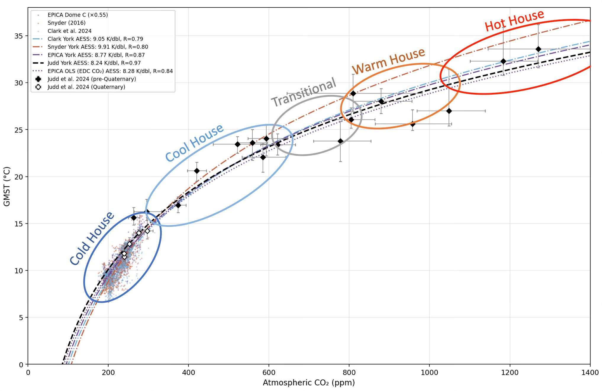
ESS however takes tens of millennia to settle out, so using it to predict temperature rises on human timescales is not really much help. Today we have increased the CO₂ concentration by a little more than 50% since pre-industrial times, but temperatures have so far only risen by ~1.5ºC, not the 4.5ºC that ESS would imply.

Instead, scientists turn to something called Equilibrium Climate Sensitivity (ECS). This value is still logarithmic but only includes the fast feedbacks, not the longer term ones. This makes it more useful since it can predict temperature responses on a decadal timescale.

So far so good, but unfortunately it turns out to be very difficult to determine a solid value for ECS. The IPCC’s latest report has the likely range between 2.5º and 4ºC, with a best estimate of 3ºC. Recent works by Tierney² and Hansen³ have independently arrived at best estimates in the 4.5-6.5ºC range.

To make matters worse, there is some evidence that although ESS stays constant, since the nature of feedbacks change in different climate states, ECS is larger in warmer states than cooler ones, for example a hot house state has no ice to melt. This makes comparisons with paleoclimates difficult. Tierney finds an ECS of 6.5ºC for the hot house PETM but 4.8ºC for the cool house Pliocene.

The difference between the IPCC’s best estimate and those of Hansen and Tierney are stark. They would mean that instead of temperatures stabilising at ~1.5ºC if we stopped emissions today, they would continue to rise to ~2.4ºC in short order. Given that the Institute and Faculty of Actuaries, and others, point to 44-88% GDP destruction at 3ºC⁴, this is something that needs to be bottomed out, and soon.

There is also evidence that ECS is rate dependent (how fast CO₂ concentrations are rising). Ocean stratification is an example of a phenomena being driven by the rate of heat uptake, trapping heat at the surface where it has a greater influence on air temperatures. Slower warming would allow the heat to be mixed into the deeper ocean, reducing the atmospheric take-up. Same final CO₂ concentration, but different initial temperature response.

As we move deeper into the 21st century, it is becoming clear that ECS is an incomplete yardstick. It treats the Earth as a passive recipient of greenhouse gases, rather than a dynamic system whose very “sensitivity” is not only driven by feedbacks, but also being altered by a range of other human activities.

Anthropogenic Efficacy

As our influence on the planet diversifies, treating the Earth’s response as a singular, CO₂ driven constant is becoming increasingly insufficient. We are simultaneously changing the biosphere and the landscape. We are emitting other pollutants that act to both warm and cool the planet, but these aren’t captured in a simple CO₂ only ECS value. CO₂ Equivalents (CO₂e), which treats other gases as having a relative CO₂ value also fail to capture all these other human influences effectively.

We should instead view climate response through the lens of Anthropogenic Climate Sensitivity (ACS): a framework where the baseline sensitivity of the Earth system is modified by specific human “multipliers.” These dictate how efficiently the Earth responds to the added heat.

In formal thermodynamics, not all units of energy (forcings) are created equal.⁵⁶⁷ In an ACS framework, a multiplier represents what scientists call an Efficacy Factor. If CO₂ has an efficacy of 1.0, other human activities can be more or less “efficient” at warming the planet per unit of energy they add.

ACS = ECS_baseline × ∑( Forcing_i × μ_i )

Where μ represents the specific multiplier for each anthropogenic driver i. Some have direct radiative effects which can be captured through Effective Radiative Forcing (ERF) but many others escape this method.

The Primary Multipliers

The Cooling Masks: Aerosols and Irrigation

Humanity doesn’t just warm the planet; we also apply “brakes” to that warming, though often unintentionally.

Sulphate Aerosols (μ≈0.6–0.9): Industrial pollution creates a “haze” that reflects sunlight. This acts as a dampening multiplier, masking the true sensitivity of the climate. If these aerosols were removed, the “unmasked” warming would surge. As pollution is reduced, this multiplier will tend towards 1.0 over the coming decades. The reduction of aerosol emissions from shipping fuels is widely believed to be partially responsible for recent ocean warming accelerations.

Agricultural Irrigation (μ≈0.9): By artificially wetting vast tracts of land, we shift energy into latent heat (evaporation) rather than sensible heat (temperature rise), providing a slight regional cooling efficacy. This practice also masks underlying warming. When aquifers run dry and the practice stops, it drives local heat up further, potentially worsening the drought.

The Feedback Primers: Land Use and Soot

Some human activities act as “force multipliers” by directly triggering the planet’s most sensitive feedback loops.

The Bowen Ratio Shift (μ≈1.1–1.3): Deforestation does more than release carbon. By replacing high-transpiration forests with dry pasture or crops, we alter the Bowen Ratio. With less water to evaporate, the surface converts solar energy directly into heat, effectively increasing the local climate sensitivity.

Natural aerosol decline (μ≈1.2–1.8): Aerosols are essential as cloud condensation nuclei but deforestation, changes in farming and land management, and crucially ocean health and pollution are reducing their production. Lower cloud cover and cloud dimming as a result reduces albedo leading to direct warming as well as less rainfall, which in turn reduces evaporation and further Bowen Ratio changes.

Black Carbon on Snow (μ≈1.5–3.0): Soot falling on the Arctic is perhaps the most potent regional multiplier. It doesn’t just trap heat in the air; it darkens the ice, triggering the ice-albedo feedback. This makes soot significantly more “efficient” at driving global melt than an equivalent amount of CO₂. Recent work suggests that micro-plastic pollution also has a similar role, both in the air and within the ocean surface layers.⁸

The Modern Additions: Aviation, Methane and Ozone

Aviation Contrails (μ≈1.2): High-altitude contrails act as artificial cirrus clouds. While they reflect some sun, their ability to trap outgoing heat gives them a high warming efficacy.⁹ This is made worse with night flights since the solar reflection aspect is not present. (Not to be confused with so called “chemtrails” which is a baseless conspiracy theory)

Methane’s Chemical Tail (μ≈1.45): Methane is a potent gas, but its multiplier is high because it chemically produces ozone and stratospheric water vapour as it decays. These are both greenhouse gasses so our emissions add “bonus” warming layers to its initial greenhouse impact.

Stratospheric ozone depletion (μ≈0.5-0.8): While ozone depletion is a significant concern, it does create a cooling efficacy since ozone is a greenhouse gas. Its depletion in the stratosphere has historically provided a slight cooling offset, particularly in the Southern Hemisphere, by allowing more long-wave radiation to escape to space.¹⁰

Even moving to a green hydrogen economy leads to hydrogen leakage, which inhibits methane destruction in the atmosphere creating an amplifying multiplier if we were to take this path. Fortunately basic economics will likely prevent this.

The Rate and State Problem

Traditional ECS assumes a slow move toward a distant equilibrium. But human influence is fast and messy. There is a rate dependency not just in terms of feedbacks such as ocean warming but also between different emissions. High-efficacy forcings, like aerosols, react in days, while CO₂ reacts over centuries. This creates a transient sensitivity that can look much higher or lower than the theoretical equilibrium.

A pattern effect also exists. Where we act matters. A multiplier isn’t just about what we do, but where. Forcings in the tropics or the Arctic have higher leverage over the global temperature than those in the mid-latitudes since they disproportionally affect evaporation and cloud forming in terms of the tropics and albedo at high latitudes.¹¹

The Socio-Economic Crossroads: SSP2-4.5 vs. SSP3-6.0

The ACS framework also reveals how different socio-economic pathways (SSPs), or emissions scenarios fundamentally change the Earth’s effective sensitivity. This in turn changes the outcomes adding more emphasis for the need to choose the safest trajectories and the right policies to achieve them.

SSP2-4.5 (The Middle Road): This pathway manages a slow unmasking of the dampening multipliers. As we gradually reduce pollution, the aerosol multiplier slowly moves toward 1.0. Because the transition is managed, we hopefully avoid termination shocks with rapid warming and the ACS stays relatively close to the baseline. This pathway also sees methane emissions gradually reduce, lowering this warming multiplier. Land use change also slows, hopefully the Bowen Ratio avoids biosphere tipping points. The end result is a predictable steady climb in temperatures where ACS stays close to baseline ECS.

This is not great though, temperatures continue to rise with all the effects of a growing climate crisis, but without catastrophic rapid changes.

SSP3-6.0 (Regional Rivalry): This is the “Multiplier Trap” since it maximises the amplifying multipliers while keeping the dampening multipliers for longer, masking the true warming. High nationalism leads to dirty energy use, keeping the aerosol mask heavy (μ≈0.65) while methane and deforestation run rampant (μ≈1.45 and 1.3). This creates a “spring-loaded” climate: a massive amount of hidden warming is suppressed by pollution, waiting for a tipping point to release it. This pathway is characterised by significant land-use change and rapid deforestation. This shifts the energy balance toward sensible heat across vast areas (the Amazon, Congo, SE Asia), effectively “priming” the local climate to react more violently to CO₂ increases.

The Net Result is that SSP3-6.0 has a higher “Hidden Sensitivity.” The gap between the observed temperature and the “latent” temperature (what would happen if the aerosols cleared) is much wider than in SSP2-4.5. Both have a time limit where climate damage reaches such a level that humanity is forced to react, either voluntarily, or through collapse. The pathway we take between now and at that point, therefore has a huge impact on the fall out and potential for recovery.

Tipping Points

Humanities choice of pathway also influences tipping point thresholds. These are often not just critical temperature points, but are influenced by other factors, factors that are also multipliers in the ACS framework.

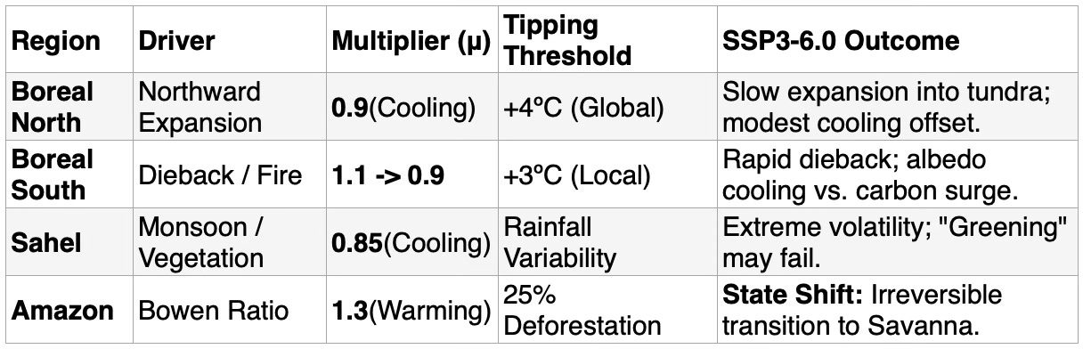
The Amazon is a good example. A recent paper from the Potsdam Institute for Climate Impact shows that deforestation, making changes to the Bowen Ratio multiplier, lowers the temperature threshold for collapse.¹² Without deforestation, the Amazon could survive 4ºC of warming, but when a critical level of deforestation (22-28%) is reached, that temperature thresholds drops to less than 2ºC. Essentially the point where the two lines cross spikes the land use multiplier. The energy partition shifts so heavily toward sensible heat that the regional atmosphere dries out, extending the dry season by 4–5 weeks and preventing the forest from recycling moisture. Current levels are about 18%.

Under an SSP2-4.5 scenario, deforestation is curtailed, keeping the multiplier around 1.1 for much longer, possibly forever. Under SSP3-6.0 the multiplier climbs to 1.3+ as deforestation exceeds 25%. This in conjunction with failure to lower methane emissions elevates the ACS to the point where the Amazon collapses in the 2040s under this pathway.

Similar observations affect the southern boreal forest die-back, but it may actually provide a negative feedback for Sahel greening. Increasing CO₂ together with southerly moving monsoon patterns could lead to a greening multiplier of 0.85-0.95 as evapotranspiration and local Bowen ratios improve.

Net-Zero and True-Zero

The ACS framework also creates insights into the net-zero goal. It reveals a fundamental tension in climate policy: the difference between stopping emissions entirely and simply “balancing the books.” In the multiplier framework, these two paths lead to very different “effective” sensitivities during the critical 2030–2050 window.

Net-zero allows for residual emissions such as aviation, cement and heavy industry as long as they are balanced by Carbon Dioxide Removal (CDR) such as direct air capture and reforestation. The danger highlighted by this framework is that replacing 1 tonne of CO₂ emission with 1 tonne of removal may not balance the multipliers. The CO₂ may be balanced, but aerosol and soot emissions may continue that are not accounted for. The results would be a smooth temperature curve with less volatility, but a higher risk of “sensitivity creep” if the high-multiplier gases (Methane, Soot) aren’t prioritised over simple CO₂ math.

True-zero or an absolute clean up implies a total cessation of all human emissions with no offsets, no carbon removal, no excuses. Depending on the rate of achieving it, the reduction in aerosols would match the reduction in methane so ACS could fairly quickly revert to baseline ECS. This is because both aerosols and methane are short-lived climate pollutants, an absolute halt to emissions causes both multipliers to drop out simultaneously, preventing a catastrophic thermal spike. This is more of a total civilisational collapse scenario than a managed transition though.

Net-zero will be a delicate balancing act where we must ensure the high-multiplier influences (like methane and deforestation) are phased out faster than the low-multiplier ones (like aerosols) to avoid a sensitivity-driven overshoot. ACS provides a metric for this that simple carbon reduction accounting misses.

Overshoot and CDR

Now that it is obvious to everyone that the lower Paris 1.5ºC target will be breached, the conversation has moved to overshoot and recovery. How little time can we spend above 1.5º, what maximum temperature will be encountered and how do we get back below it? To that end the new pathways for CMIP7 and the next IPCC round of reports have been suggested.¹³ There are seven in total that replace the SSP range discussed above. All but two of them include huge levels of Carbon Dioxide Removal (CDR) as they are designed to limit temperatures to within the Paris goals (2ºC by 2100).

The ACS framework introduces a vital aspect to this recovery, that of the asymmetry of cooling.

When we pull carbon out of the atmosphere using Carbon Dioxide Removal, the planet does not simply reverse the warming track it took on the way up. The multipliers behave differently when emissions are net-negative compared to when they were rising. This asymmetry is central to calculating how hard, fast, and long we have to deploy negative emissions to stabilise or lower global temperatures.

Through the lens of ACS, we can extract several critical insights regarding overshoot recovery:

The Hysteresis Trap: Multiplier Asymmetry

The assumption built into many simple climate models is that if you remove 1 ppm of CO₂, you undo the exact amount of warming that 1 ppm caused. In reality, Earth system components exhibit hysteresis—a lag or permanent change in response.

In the ACS framework, the multipliers are state-dependent. On the way down, the “initial climate state” has been altered by the peak of the overshoot:

The Carbon Sink Weakening Multiplier (μsink >1.0 on the way down): When CO₂ was rising, the ocean and land biosphere absorbed roughly half our emissions (the solubility and fertilisation pumps). During net-negative emissions, however, the ocean and land start releasing stored CO₂ back into the atmosphere to maintain equilibrium. CDR has to work twice as hard because it is fighting a “burping” planet.

The Albedo Memory Loss (μalbedo >1.0 on the way down): If an overshoot melts a major ice sheet or thins the Arctic pack ice, lowering the temperature via negative emissions does not instantly refreeze that ice. The dark ocean or land remains exposed, meaning the albedo multiplier stays stubbornly high long after the CO₂ concentration drops.

The Bowen Ratio Permanence (The Irreversible Amazon Shift)

If an overshoot triggers a tipping point, like the 22%–28% deforestation limit in the Amazon or a major Boreal dieback, the regional multiplier changes permanently. During Rising Emissions, μland_use creeps up as forest is cleared, converting latent heat to sensible heat. During Net-Negative Operations, even if we deploy high-tech Direct Air Capture (DAC) to lower global CO₂, it doesn’t automatically replant the Amazon or heal a scorched Siberian Taiga. The biome has permanently shifted to a savanna or steppe state.

The lesson from ACS is that a permanently damaged biome fixes the regional Bowen Ratio multiplier at a high level. Thus, the post-overshoot ACS remains higher than the pre-overshoot baseline, meaning the planet will remain warmer for a given level of CO₂ than it was in the 20th century. The IPCC suggest returning to 350ppm of CO₂ will create a safe climate, ACS begs to differ, if anything levels even lower than the pre-industrial 280ppm may be required for a significant period to return the cryosphere to a stable state.

CDR Strategy: Matching Method to Multiplier

Not all net-negative strategies are equal. The ACS framework implies that instead of just pulling generic carbon equivalents out of the sky, CDR must target specific, high-leverage multipliers to optimise cooling such as:

High-Efficacy Methane Removal: Because methane dictates short-term rate dependencies and has an expanded chemical efficacy multiplier, targeted atmospheric methane destruction yields immediate dividends. Stripping a ton of methane drops the effective ACS much faster during an overshoot than stripping an equivalent radiative unit of CO₂.

Enhanced Ocean Alkalinity, when applied directly to the ocean, or on large coastal agricultural scales this changes ocean alkalinity allowing it to absorb more CO₂. This directly counteracts the weakening ocean sink multiplier (μsink ), preventing the ocean from outgassing its stored carbon back into the atmosphere during the ramp-down phase.

Bio-Energy with Carbon Capture and Storage (BECCS) removes CO₂ by growing crops which are then processed and burned for power generation, but with the emissions captured and permanently sequestered. This would have a positive influence on ACS since any Bowen ratio improvement through crop evapotranspiration would be in addition to the CO₂ removal. This is assuming that the land to grow the crops was not cleared forest. In fact the multiplier would have to be based on the alternative use for the land. More cooling may be achieved through reforestation than using the land for BECCS, regardless of the CO₂ reduction.

Designing the Overshoot Recovery Equation

Using ACS for overshoot analysis teaches us that “cooling is not simply warming in reverse.” The paths are asymmetrical, and a temporary thermal overshoot leaves permanent scars on the Earth’s feedback mechanisms, meaning the planet we return to will possess a fundamentally altered climate sensitivity.

Even more complexity could be added if we resort to Solar Radiation Management as an emergency cooling measure. That too will have to be carefully managed to ensure the multipliers are considered as part of the design and monitoring.

Conclusions

Climate change is often discussed in terms of how much carbon. The ACS framework argues it is also a matter of how much sensitivity. The ECS is a vital theoretical yardstick, but the Anthropogenic Climate Sensitivity, the ECS as modified by our specific suite of multipliers, is what we actually live through. By quantifying these factors, we move away from a world where we simply “wait and see” how the planet warms, and into a world where we can precisely identify which human levers are the most dangerous to pull and manage their release in an orderly transition.

By understanding that our actions—from the way we farm to the altitude at which we fly—directly tune the Earth’s responsiveness, we gain a more nuanced view of the risks ahead.

Due to current aerosol emissions and lags within the system, we are currently in a climate debt, apparently unaware of the true balance of our account. The ACS framework provides a way of attributing this and other multipliers to calculate the value of this subsidy, and how to pay it back.

We are not just changing the temperature; we are changing the very rules by which the Earth’s climate operates. To navigate the 21st century, we may need to manage the multipliers as aggressively as we manage the emissions.

So what is the result? Proper data needs to be collected to calculate each multiplier, but a back of the envelope estimate, based on the numbers shown above suggest an ACS of ~1.8 x ECS. So using IPCC’s 3ºC gives us a current ACS of ~5.4ºC. That suggests a stable temperature of +2.7ºC for our emissions and actions to date, once the energy balances out. That’s not unreasonable given how hard the Earth is trying to warm as the energy imbalance continues to climb. If we were to achieve net or true zero, however the methane and aerosol multipliers would slide back to 1.0 leaving legacy deforestation and other long term pollutants alone. Temperatures could then settle out at ~1.7ºC. Food for thought.

If you found this article interesting or useful (and not too nerdy), please tick the ❤️ button as it helps the algorithm point more people in this direction and gives us feedback on what subjects are most useful. Thank you!

1.

2. J.E. Tierney et al., Spatial patterns of climate change across the Paleocene–Eocene Thermal Maximum, Proc. Natl. Acad. Sci. U.S.A. 119 (42) e2205326119, https://doi.org/10.1073/pnas.2205326119 (2022).

3. James E Hansen et al., Global warming in the pipeline, Oxford Open Climate Change, Volume 3, Issue 1, 2023, kgad008, https://doi.org/10.1093/oxfclm/kgad008

4.

5. Hansen, J., et al. (2005), Efficacy of climate forcings, J. Geophys. Res., 110, D18104, doi:10.1029/2005JD005776. https://agupubs.onlinelibrary.wiley.com/doi/10.1029/2005JD005776

6. Richardson, T. B., Forster, P. M., Smith, C. J., Maycock, A. C., Wood, T., Andrews, T., et al. (2019). Efficacy of climate forcings in PDRMIP models. Journal of Geophysical Research: Atmospheres, 124, 12824–12844. https://doi.org/10.1029/2019JD030581

7. Weitzman, M. L. (2009). On Modeling and Interpreting the Economics of Catastrophic Climate Change. Review of Economics and Statistics, 91(1), 1–19. https://dash.harvard.edu/server/api/core/bitstreams/7312037c-728a-6bd4-e053-0100007fdf3b/content

8. Liu, Y., Fu, H., Zhang, H. et al. Atmospheric warming contributions from airborne microplastics and nanoplastics. Nat. Clim. Chang. 16, 598–605 (2026). https://doi.org/10.1038/s41558-026-02620-1

9. Teoh, R., Engberg, Z., Schumann, U., Voigt, C., Shapiro, M., Rohs, S., and Stettler, M. E. J.: Global aviation contrail climate effects from 2019 to 2021, Atmos. Chem. Phys., 24, 6071–6093, https://doi.org/10.5194/acp-24-6071-2024, 2024.

10. Egorova T, Rozanov E, Arsenovic P, Peter T and Schmutz W (2018) Contributions of Natural and Anthropogenic Forcing Agents to the Early 20th Century Warming. Front. Earth Sci. 6:206. doi:10.3389/feart.2018.00206

11. Myhre G, Byrom RE, Andrews T, Forster PM and Smith CJ (2024) Efficacy of climate forcings in transient CMIP6 simulations. Front. Clim. 6:1397358. doi:10.3389/fclim.2024.1397358

12. Wunderling, N., Sakschewski, B., Rockström, J. et al. Deforestation-induced drying lowers Amazon climate threshold. Nature (2026). https://doi.org/10.1038/s41586-026-10456-0

13. Van Vuuren, D. P.et al. : The Scenario Model Intercomparison Project for CMIP7 (ScenarioMIP-CMIP7), Geosci. Model Dev., 19, 2627–2656, https://doi.org/10.5194/gmd-19-2627-2026, 2026.